IFERROR In Excel

What is IFError?

A common request in the area of functions is something to simplify error checking.

e.g If user wants to catch the errors in VLOOKUP and use their own error text opposed to excel error, they can use IF and ISERROR functions or user can use only IFERROR.

Here are both the examples.

1) In first example we will try to get Name Value from left grid by using IF and ISERROR.

 =IF(ISERROR(VLOOKUP(D5,A$2:B$6,2,FALSE)),"Value is not Availble in Source Table",VLOOKUP(D5,A5:B9,2,FALSE))

 

 2) For same scenario we are using IFERROR.

=IFERROR(VLOOKUP(D7,A2:B7,2,FALSE),"Value is not Availble in Source Table")

 

 

As you can see that both are providing same result, but user need to repeat the VLOOKUP formula twice. This has a number of problems

a) First, it is hard to maintain.. if you have to change the formula you have to do two time

b) Second, it can affect the performance because formulas are quite often run twice.

 

Keep Reading and Happy Diwali

Sanjay Bakshi

mesanjaybakshi@gmail.com

 

 

Slicer in Excel 2010

In earlier versions of Microsoft Excel, we can use report filters to filter data in a PivotTable report, but it is not easy to see the current filtering state when you filter on multiple items. In Microsoft Excel 2010, you have the option to use slicers to filter the data. Slicers provide buttons that you can click to filter PivotTable data. In addition to quick filtering, slicers also indicate the current filtering state, which makes it easy to understand what exactly is shown in a filtered PivotTable report.

Slicers are easy-to-use filtering components that contain a set of buttons that enable you to quickly filter the data in a PivotTable report, without the need to open drop-down lists to find the items that you want to filter.

When we use a regular PivotTable report filter to filter on multiple items, the filter indicates only that multiple items are filtered, and we have to open a drop-down list to find the filtering details. However, a slicer clearly labels the filter that is applied and provides details so that you can easily understand the data that is displayed in the filtered PivotTable report.

Slicers are typically associated with the PivotTable in which they are created.

When we create any slicer we get the following elements

1. A slicer header indicates the category of the items in the slicer.

2. A filtering button that is not selected indicates that the item is not included in the filter.

3. A filtering button that is selected indicates that the item is included in the filter.

4. A Clear Filter button removes the filter by selecting all items in the slicer.

5. A scroll bar enables scrolling when there are more items than are currently visible in the slicer.

 

 

Selection of Slicer

 

 

Slicer Output

 

 

Keep Learning

Sanjay Bakshi

mesanjaybakshi@gmail.com

Excel 2010 - Some Important Information

Microsoft Excel is a spreadsheet application developed by Microsoft for Microsoft Windows and Mac OS. It features calculation, graphing tools, pivot tables, and a macro programming language called Visual Basic for Applications. Microsoft has done minor enhancements and 64 bit support also

 

ü You can undo the last 100 actions

ü Each worksheet holds 1,048,576 rows by 16,384 columns

ü There are 1,024 global fonts available to use, 512 per worksheet

ü Zoom range is from 10 percent to 400 percent

ü You can select 2,147,483,648 cells that are not touching

ü You can have up to 255 arguments in a function

ü You can nest 64 levels of functions per formula

ü You can have up to 255 data series in one chart

ü You can highlight 32,767 cells per worksheet

ü Multi-threading recalculation (MTR) for commonly used functions

ü Improved pivot tables

ü More conditional formatting options

ü Additional image editing capabilities

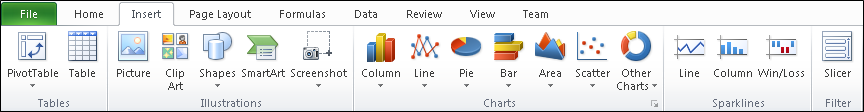
ü In-cell charts called spark lines

ü Ability to preview before pasting

ü Many new formulas, most highly specialized to improve accuracy

 

Keep Learning

Sanjay Bakshi

mesanjaybakshi@gmail.com

 

Sparkline in Excel 2010

A Sparkline is a small chart that is aligned with rows of some tabular data and usually shows trend information.

1.     Select the data from which you want to make a Sparkline.

2.     Go to Insert > Sparkline and select the type of Sparkline

3.     Specify a target cell where you want the Sparkline to be placed

4.     Optional: Format the Sparkline if you want.

There are 3 basic types of Sparkline in Excel 2010.

1.     Line chart

2.     Column chart

3.     Win-loss chart.

 

 

Selection of Sparkline (Last Set)

 

Data Selection for Sparkline

 

Sparkline Formatting

 

Keep Learning
Sanjay Bakshi
mesanjaybakshi@gmail.com
 

Unique Records in Excel

Remove Dupes in a column: Data Menu>Filter>Advanced Filter. Check Copy to another location (select a Copy To range). Unique records only.

Thanks,
Sanjay Bakshi
mesanjaybakshi@gmail.com

@@ RowCount

@@ RowCount

It returns the number of rows affected by the last statement. If numbers are more than 2 billion then we have to use @@ ROWCOUNT_BIG.

The return value of this will be in Integer data type.

USE <DB Name>

GO

UPDATE <Table Name>

 SET <Column Value> = “Value”

IF @@ROWCOUNT = 0

PRINT 'Warning: No rows were updated';

GO

USE <DB Name>

GO

Insert into <Table Name> (Col1, Col2) values (‘Val1 for Col1’,’ Val1 for Col2’)

Select @@RowCount

GO

Keep Learning

Sanjay

mesanjaybakshi@gmail.com

Share Point Installation

Hi All,

Please find the Installation Details of Share Point.

https://drive.google.com/file/d/0B13PrmqQdIU_Tm5XOEhrbGZFWFk/view?usp=sharing

Thanks,
Sanjay Bakshi